01 / 37
// Imaging in Paris · IHP · 05/12/2026

Toward One-Step Image Restoration
with Generative Priors

From Plug-and-Play Diffusion to Flow Distillation
$$\mathbf{y} = \mathcal{H}(\mathbf{x}) + \mathbf{n} \;\;\longrightarrow\;\; \hat{\mathbf{x}}$$
Yuanzhi Zhu
Diffusion Models · Flow Matching · Image Restoration
Imaging in Paris Seminar · Institut Henri Poincaré
DiffPIR · CVPRW 2023
OFTSR · ICLR 2026
MFSR · arXiv 2026
02 Roadmap

A Research Journey

Part I · 2023
DiffPIR
Multi-step Diffusion
Plug-and-Play IR
~100 NFEs
Part II · 2024
OFTSR
One-step Flow SR
Tunable Trade-off
1 NFE
Part III · 2025
MFSR
MeanFlow Distillation
Real-World SR
1 NFE
Progressive efficiency: 100 steps → 1 step (with tunable fidelity ↔ realism trade-off).  Progressive generality: synthetic → real-world.
03 Background

Image Restoration as an Inverse Problem

// Forward degradation model $$\mathbf{y} = \mathcal{H}(\mathbf{x}) + \mathbf{n}$$
  • $\mathbf{y}$: observed degraded image
  • $\mathcal{H}$: degradation operator (blur, downsampling, masking)
  • $\mathbf{n}$: additive noise
  • Goal: recover $\mathbf{x}$ from $\mathbf{y}$
Tasks
Super-Resolution · Deblurring · Inpainting
Challenge
Ill-posed: many $\mathbf{x}$ explain the same $\mathbf{y}$
04 Background

Plug-and-Play Image Restoration

// MAP estimation with explicit prior $$\hat{\mathbf{x}} = \arg\min_{\mathbf{x}} \;\underbrace{\frac{1}{2}\|\mathbf{y} - \mathcal{H}(\mathbf{x})\|^2}_{\text{data fidelity}} + \underbrace{\lambda \, \Phi(\mathbf{x})}_{\text{prior}}$$
HQS Splitting
  • 1.Data subproblem: proximal step on $\|\mathbf{y}-\mathcal{H}(\mathbf{x})\|^2$
  • 2.Prior subproblem: apply denoiser $\mathcal{D}_\sigma$
KEY INSIGHT
Any denoiser can serve as an implicit image prior. Replace $\Phi(\mathbf{x})$ with a denoiser — no need to define the prior explicitly.
05 Background

Diffusion Models are Powerful Priors

Forward Process
Gradually add Gaussian noise: $\mathbf{x}_0 \to \mathbf{x}_1 \to \cdots \to \mathbf{x}_T \sim \mathcal{N}(0, \mathbf{I})$
Reverse Process
Learn to denoise: $\mathbf{x}_t \to \mathbf{x}_0$. The denoiser $D_\theta(\mathbf{x}_t, t)$ predicts clean $\mathbf{x}_0$ from noisy $\mathbf{x}_t$.
Score ↔ Denoiser (Tweedie)
$$\nabla_{\mathbf{x}_t}\!\log q(\mathbf{x}_t) = \frac{\sqrt{\bar\alpha_t}\,D_\theta(\mathbf{x}_t, t) - \mathbf{x}_t}{1 - \bar\alpha_t}$$
WHY DIFFUSION FOR IR?
  • Diffusion models provide a family of denoisers at different noise levels
  • This naturally matches PnP where denoiser strength decreases over iterations
  • Much richer generative capacity with scaled-up denoisers — the sampling schedule is very important
06 Preliminaries
DDPM

DDPM: Forward Process

// Gradually add noise over $T$ steps $$q(\mathbf{x}_t|\mathbf{x}_{t-1}) = \mathcal{N}\!\left(\mathbf{x}_t;\, \sqrt{1-\beta_t}\,\mathbf{x}_{t-1},\, \beta_t \mathbf{I}\right)$$
// Closed-form for arbitrary $t$ (skip steps) $$\mathbf{x}_t = \sqrt{\bar\alpha_t}\,\mathbf{x}_0 + \sqrt{1-\bar\alpha_t}\,\boldsymbol{\epsilon}, \quad \boldsymbol{\epsilon}\sim\mathcal{N}(0,\mathbf{I})$$
  • $\beta_t$: noise schedule
  • $\alpha_t = 1 - \beta_t$, $\;\bar\alpha_t = \prod_{i=1}^{t}\alpha_i$
  • As $t\to T$: $\bar\alpha_T \approx 0$, so $\mathbf{x}_T \sim \mathcal{N}(0, \mathbf{I})$
The forward process destroys structure; the reverse process must learn to recover it.
07 Preliminaries
DDPM

DDPM: Reverse Process & Training

// Learned reverse step $$p_\theta(\mathbf{x}_{t-1}|\mathbf{x}_t) = \mathcal{N}\!\left(\mathbf{x}_{t-1};\, \boldsymbol{\mu}_\theta(\mathbf{x}_t, t),\, \sigma_t^2\mathbf{I}\right)$$
// Simple denoising objective (predict the noise) $$L_{\text{simple}} = \mathbb{E}_{\mathbf{x}_0,\boldsymbol{\epsilon},t}\!\left[\|\boldsymbol{\epsilon} - \boldsymbol{\epsilon}_\theta(\mathbf{x}_t, t)\|^2\right]$$
DENOISER = SCORE
The noise predictor $\boldsymbol{\epsilon}_\theta$ is equivalent to the score function: $$\nabla_{\mathbf{x}_t}\!\log q(\mathbf{x}_t) = -\frac{\boldsymbol{\epsilon}_\theta(\mathbf{x}_t,t)}{\sqrt{1-\bar\alpha_t}}$$
EQUIVALENT PREDICTIONS
Predict noise $\boldsymbol{\epsilon}$, clean image $\mathbf{x}_0$, score $\nabla\!\log q(\mathbf{x}_t)$, or velocity $\mathbf{v}$
08 Preliminaries
Flow Matching

Flow Matching / Rectified Flow (Simple Schedule)

// Learn a velocity field that transports noise → data $$\frac{d\mathbf{x}_t}{dt} = \mathbf{v}_\theta(\mathbf{x}_t, t), \quad t \in [0, 1]$$
// Conditional flow matching loss $$L_{\text{CFM}} = \mathbb{E}_{t,\,\mathbf{x}_0,\,\mathbf{x}_1}\!\left[\|\mathbf{v}_\theta(\mathbf{x}_t, t) - (\mathbf{x}_1 - \mathbf{x}_0)\|^2\right]$$
LINEAR INTERPOLATION
$$\mathbf{x}_t = (1-t)\,\mathbf{x}_0 + t\,\mathbf{x}_1$$
TARGET VELOCITY
$$\frac{d\mathbf{x}_t}{dt} = \mathbf{x}_1 - \mathbf{x}_0$$
09 I · DiffPIR
CVPRW 2023

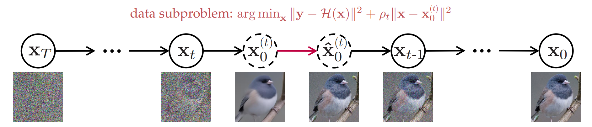
DiffPIR Denoising Diffusion Models for Plug-and-Play Image Restoration

DiffPIR pipeline illustration

Yuanzhi Zhu, Kai Zhang, Jingyun Liang, Jiezhang Cao, Bihan Wen, Radu Timofte, Luc Van Gool

  • General framework for SR, deblurring, inpainting
  • Training-free: no task-specific training, just an off-the-shelf diffusion model
  • Strong perceptual quality on FFHQ & ImageNet
10 I · DiffPIR
Method

HQS Formulation

// Data subproblem (closed-form for linear H) $$\hat{\mathbf{x}}_0^{(t)} = \arg\min_{\mathbf{x}} \;\|\mathbf{y} - \mathcal{H}(\mathbf{x})\|^2 + \rho_t \|\mathbf{x} - \tilde{\mathbf{x}}_0^{(t)}\|^2$$
  • 1.Predict $\tilde{\mathbf{x}}_0$ from noisy $\mathbf{x}_t$ via score model
  • 2.Solve data subproblem: enforce consistency with $\mathbf{y}$
  • 3.Diffuse back: one reverse diffusion step → $\mathbf{x}_{t-1}$
KEY PARAMETER
$\rho_t$ controls data fidelity weight — increases over time as denoiser noise decreases
11 I · DiffPIR
Algorithm

Algorithm Walkthrough

DiffPIR Algorithm 1
  • Start from pure noise $\mathbf{x}_T \sim \mathcal{N}(0, \mathbf{I})$
  • At each step $t$: predict clean $\tilde{\mathbf{x}}_0$ via the diffusion denoiser
  • Solve data subproblem (closed-form for linear $\mathcal{H}$)
  • Perform one reverse diffusion step → $\mathbf{x}_{t-1}$
Works with any linear $\mathcal{H}$ — just change the data step
12 I · DiffPIR

Key Design Choices

Noise Schedule Alignment
Diffusion noise level matches PnP denoiser strength at each iteration
Pretrained Model
No task-specific fine-tuning — uses off-the-shelf diffusion model trained on ImageNet
Sub-sampled Schedule
100 NFEs (sub-sampled from 1000) — enough for high-quality restoration
Versatility
Same framework for SR, deblurring, inpainting — just change $\mathcal{H}$
13 I · DiffPIR
Qualitative Results

One Framework, Three Tasks

Super-Resolution
DiffPIR SR qualitative results on FFHQ

4× downsampled FFHQ

Deblurring
DiffPIR deblurring results

Motion & Gaussian blur

Inpainting
DiffPIR inpainting results

Box & random mask

Same pretrained diffusion model — only the operator $\mathcal{H}$ changes between tasks.

14 I · DiffPIR
Summary

DiffPIR: Summary

Strengths
  • +General framework for multiple IR tasks
  • +Strong perceptual quality (SOTA on FFHQ/ImageNet)
  • +No task-specific training
Limitations
  • ~100 NFEs per image — slow inference
  • Requires known degradation model $\mathcal{H}$
  • Theory–practice gap for training-free methods
Can we achieve similar quality in one single step?
15 Transition · I → II

The Speed Problem

MethodSteps (NFEs)Quality
DiffPIR100SOTA
DDRM20Good
DPS1000Good
One-step?1???

Practical deployment needs cheap inference. Distillation is the standard answer: compress a multi-step teacher into a one-step student.

16 II · OFTSR
ICLR 2026

OFTSR One-Step Flow for Image Super-Resolution with Tunable Fidelity-Realism Trade-offs

OFTSR overview with tunable outputs

Yuanzhi Zhu*, Ruiqing Wang*, Shilin Lu, Junnan Li, Hanshu Yan, Kai Zhang

  • One-step flow-based super-resolution
  • Tunable fidelity-realism trade-off at inference
  • SOTA one-step SR on FFHQ, DIV2K, ImageNet
17 II · OFTSR
Method

Two-Stage Framework

STAGE 1: Train Teacher
Conditional rectified flow model for SR. Multi-step sampling with noise-augmented LR inputs.
STAGE 2: Distill Student
One-step student via trajectory-aligned distillation. Force student predictions to lie on teacher's ODE trajectory.
OFTSR distillation diagram
18 II · OFTSR

Noise-Augmented Conditional Flow

// Variance-Preserving (VP) noise augmentation $$\mathbf{x}_0 = \sqrt{1 - \sigma_p^2}\,\mathbf{x}_{\text{LR}} + \sigma_p\,\boldsymbol{\epsilon}$$ // then condition on $\mathbf{x}_{\text{LR}}$ via concatenation
  • Expand support of initial distribution
  • Enable diverse HR reconstructions from single LR
  • VP noise preserves LR information
WHY NOISE AUGMENTATION?
Without noise: flow collapses LR→HR mapping to a single deterministic output. With noise: learns a distribution over possible HR images, enabling tunable generation.
19 II · OFTSR
Key Innovation

Trajectory-Aligned Distillation

// (1) Teacher's ODE trajectory: $s > t$ on same path $$\mathbf{x}_s = \mathbf{x}_t + (s - t)\,\mathbf{v}_\theta(\mathbf{x}_{t,\text{LR}}, t)$$
// (2) Student's one-step predictions from $\mathbf{x}_0$ $$\mathbf{x}_t = \mathbf{x}_0 + t\,\mathbf{v}_\phi(\mathbf{x}_{0,\text{LR}}, t), \quad \mathbf{x}_s = \mathbf{x}_0 + s\,\mathbf{v}_\phi(\mathbf{x}_{0,\text{LR}}, s)$$
// (3) Substitute (2) into (1) → constraint on student $$s\bigl(\mathbf{v}_\phi^{(s)} - \mathbf{v}_\phi^{(t)}\bigr) = (s{-}t)\bigl(\mathbf{v}_\theta^{(t)} - \mathbf{v}_\phi^{(t)}\bigr)$$
FINAL DISTILLATION LOSS
$$\mathcal{L}_{\text{distill}}(\phi) = \mathbb{E}\!\left[\Bigl\|\mathbf{v}_\phi^{(s)} - \mathrm{SG}\!\Bigl[\mathbf{v}_\phi^{(t)} + \tfrac{dt}{s}\bigl(\mathbf{v}_\theta^{(t)} - \mathbf{v}_\phi^{(t)}\bigr)\Bigr]\Bigr\|^2\right]$$
where $dt = s - t$ and SG is stop-gradient (training stability)
  • Forces one-step student onto teacher's ODE trajectory
  • Discrete counterpart of forward distillation (related to MeanFlow / AlignYourFlow)
20 II · OFTSR
Unique Feature

Tunable Fidelity-Realism

OFTSR fidelity-realism tradeoff visualization
$t = 0$: high fidelity (PSNR-optimal)
$t = 1$: high realism (perceptual quality)
21 II · OFTSR
Results

Quantitative Results

OFTSR PSNR vs FID comparison

OFTSR achieves state-of-the-art one-step SR on ImageNet 256×256. Bubble size indicates NFEs — OFTSR uses only 1 NFE.

22 II · OFTSR
Comparison

Qualitative Comparisons

OFTSR qualitative comparison with other methods
23 II · OFTSR
Summary

OFTSR: Summary

Achievements
  • +One step — 100× faster than DiffPIR
  • +Tunable fidelity-realism at inference
  • +SOTA on FFHQ, DIV2K, ImageNet — also extends to real-world SR & AIGC enhancement
Limitations
  • Performance bounded by teacher model capabilities
  • Limited robustness to complex LR degradations
  • Future: GT regression / adversarial supervision, better degradation handling
Next: a framework specialized for real-world degradations.
24 III · MFSR
arXiv 2026

MFSR MeanFlow Distillation for One Step Real-World Image Super Resolution

MFSR multi-step results on real-world images

Ruiqing Wang, Kai Zhang, Yuanzhi Zhu, Hanshu Yan, Shilin Lu, Jian Yang

  • MeanFlow distillation for one-step SR
  • Designed for real-world degradations
  • Optional multi-step refinement path
25 III · MFSR
Pipeline

MeanFlow Distillation Pipeline

MFSR MeanFlow distillation pipeline

Teacher predicts instantaneous velocity $\mathbf{v}(\mathbf{z}_t, t)$. Student learns average velocity $\mathbf{u}(\mathbf{z}_t, t, s)$ over intervals.

26 III · MFSR
Comparison

Real-World Qualitative Results

MFSR qualitative comparison on real-world images
27 III · MFSR
Summary

MFSR: Summary

Achievements
  • +One-step Real-ISR with high realism & fine details
  • +Optional multi-step refinement — trade compute for quality
  • +Improved teacher CFG distillation — stronger guidance signal
  • +Strong human preference (38.9%) on real-world benchmarks
Limitations
  • Quality still bounded by the multi-step teacher (DiT4SR)
  • Specialized for SR — not yet a general restoration framework
  • Future: human/RL feedback, broader inverse problems
MeanFlow distillation: a flexible bridge between one-step efficiency and multi-step quality.
28 IV · SMFSR
ICML 2026

SMFSR Noise-Started One-Step Real-SR via SplitMeanFlow & GAN Refinement

SMFSR three paradigms: multi-step, vanilla one-step, noise-started one-step

Wei Zhu, Kai Zhang, Yu Zheng, Lei Luo, Yong Guo, Jian Yang

  • Noise-started one-step Real-SR
  • Built on SplitMeanFlow — an algebraic alternative to MeanFlow
  • GAN refinement with DINOv3 + VSD
KEY INSIGHT
Many one-step Real-SR methods (OSEDiff, TSD-SR, CTMSR) map LR → HR directly. SMFSR keeps the noise → HR paradigm — preserving stochasticity for richer textures.
29 IV · SMFSR
Method

SplitMeanFlow + GAN Refinement

SMFSR two-stage training pipeline
// Interval Splitting Consistency: any $r \le s \le t$ $$(t-r)\,\mathbf{u}_\theta(\mathbf{z}_t,r,t) = (s-r)\,\mathbf{u}_\theta(\mathbf{z}_s,r,s) + (t-s)\,\mathbf{u}_\theta(\mathbf{z}_t,s,t)$$
VS. MEANFLOW
Algebraic identity replaces JVPs — no autograd through time. Set $r=0,\,t=1$ for one-step inference.
30 IV · SMFSR
Results

SOTA Perceptual Quality on Real-SR

SMFSR qualitative comparison vs SOTA Real-SR methods
DIV2K · CLIPIQA
0.7545
vs InvSR 0.7181
DIV2K · MUSIQ
69.97
vs SeeSR 68.04
DIV2K · MANIQA
0.6611
vs InvSR 0.6424
31 Synthesis

A Unified View

AspectDiffPIROFTSRMFSRSMFSR
FrameworkPnP + DiffusionFlow MatchingMeanFlow Distill.SplitMeanFlow + GAN
Steps~10011 (+ optional multi)1
TasksSR, Deblur, InpaintSR (+ AIGC enh.)Real-world SRReal-world SR
DegradationKnown / syntheticSynthetic + Real-worldReal-worldReal-world
Start PointNoiseNoise-aug. LRNoise + LR cond.Noise + LR cond.
Key InnovationDiffusion as PnP denoiserTrajectory distillationMeanFlow averagingISC + GAN refinement
32 Conclusion

Key Takeaways

1. Diffusion and flow models are powerful priors for image restoration — far beyond discriminative denoisers
2. Progressive efficiency: 100 steps → 1 step — distillation (trajectory, MeanFlow, SplitMeanFlow) is the key enabler
3. Progressive generality: synthetic → real-world — bridging the domain gap with task-specific design
4. Design choices matter: tunable trade-offs, noise-started generation, and refinement stages all reshape the quality–efficiency frontier
33 Conclusion
Future

Future Directions

01
Test-Time Scaling
Can we adaptively allocate compute at inference? Use more steps for hard regions, fewer for easy ones — scaling quality with test-time budget.
02
Reinforcement Learning
Move beyond distillation — optimize generators directly with reward signals (perceptual quality, human preference) via RL-based fine-tuning.
03
Predictive Uncertainty
Quantify where the model hallucinates — per-object / per-region confidence maps that distinguish faithful reconstruction from plausible guesses. Critical for trustworthy use in medical, scientific, and forensic imaging.
Toward generative restoration that is fast, controllable, and self-aware — bridging distillation, RL, and uncertainty quantification.
Q&A
Yuanzhi Zhu
backup Flow Maps · A Unifying View
Bonus

OFTSR & MFSR are Flow Maps

// Flow map: maps any state at time $t$ directly to the state at time $s$ along the PF-ODE $$f_\theta(\mathbf{x}_t,\, t,\, s) \;\approx\; \mathbf{x}_s$$
PART II · OFTSR
Fixed source: $t = 0$ (noise-aug LR start)
$f_\theta(\mathbf{x}_0, 0, s) \approx \mathbf{x}_s$
Predict state at any output time $s$ from the fixed start.
PART III · MFSR
Average-velocity parameterization:
$f_\theta(\mathbf{x}_t, t, s) = \mathbf{x}_t + (s-t)\,\mathbf{u}_\theta(\mathbf{x}_t, t, s)$
Any pair $(t, s)$ — enables one-step and multi-step refinement.
Other special cases: consistency models (fixed target $s = 1$, any source $t$)  ·  flow matching ($s \to t$, instantaneous velocity).
backup Reverse Convolution · A Different Path
ICCV 2025

Reverse Convolution A True Inverse Operator for Restoration

Huang, Liu, Zhang, Tai, Yang, Zeng, Zhang — ICCV 2025
PROBLEM
Transposed convolution is not a true inverse of convolution — it just upsamples with learned filters.
// Forward: depthwise conv + downsample $$\mathbf{Y} = (\mathbf{X} \otimes \mathbf{K})\!\downarrow_s$$
// Inverse via regularized least-squares $$\mathbf{X}^{*} = \arg\min_{\mathbf{X}}\;\| \mathbf{Y} - (\mathbf{X}\otimes\mathbf{K})\!\downarrow_s\|_F^2 + \lambda\,\|\mathbf{X} - \mathbf{X}_0\|_F^2$$
CLOSED-FORM (s = 1)
$$\mathbf{X}^{*} = \mathcal{F}^{-1}\!\!\left(\frac{\overline{\mathcal{F}_K}\,\mathcal{F}_Y + \lambda\,\mathcal{F}_{X_0}}{|\mathcal{F}_K|^2 + \lambda}\right)$$
FFT-based — differentiable, $\mathcal{O}(N\log N)$.
CONNECTION
A learnable analog of the data step we saw in DiffPIR — but baked into a single CNN layer.
backup ConverseNet · Drop-in Replacement
Results

A Reverse-Conv Block for Any Network

CONVERSE2D BLOCK
Converse2D
  ↓
LayerNorm
  ↓
1×1 Conv
  ↓
GELU
Transformer-like stack — replaces conv / transposed-conv layers.
TaskDatasetConvConvTConverse
Denoise σ=25Set1230.6430.6130.70
Denoise σ=25BSD6829.3029.2929.36
SR ×4Set532.2332.0932.25
SR ×4Urban10026.2425.8926.24
DeblurBSD10032.1832.46
DeblurUrban10031.4831.96
Consistent gains across denoising · SR · deblurring — a complementary, non-generative direction for image restoration.