The Distillation in On-Policy Distillation

TL;DR

This gonna be a short blog to share some of my thoughts on the distillation in on-policy distillation (during my discussion with Yuchen Zhu), which is obvious but anyway I want to write it down as a blog post.

In one sentence, I found that the famous diffusion distillation framework (DMD, Diff-Instruct, etc.) and the recently proposed forward-process based diffusion RL fine-tuning methods are actually doing the same thing.

The Distillation in On-Policy Distillation

The Illustration of the On-Policy Generator and the Objective

As shown in the figure below, the on-policy generator is actually a model $\theta$ that take inputs noise $x_0$ and context $c$ to generate outputs $x_1$. For diffusion model, this generation can take multiple $T$ steps, using corresponding samplers such as DDIM, DPM solver or even CM sampler (for the generator trained with consistency model objective or DMD objective).

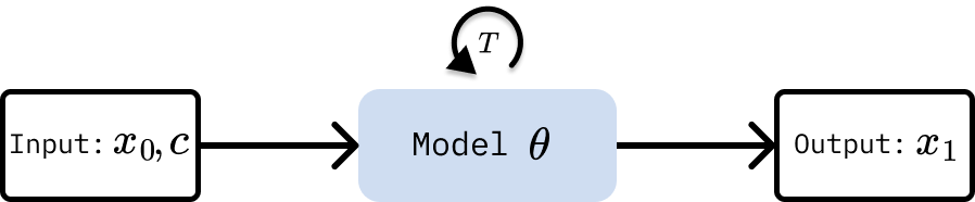
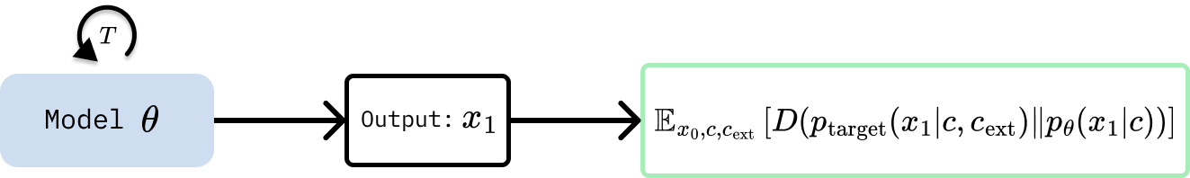
Let’s denote the generator’s output distribution as $p_\theta(x_1\mid c)$, then we can write the objective of the on-policy distillation as minimizing some divergence between the generator’s output distribution and a target distribution $p_{\mathrm{target}}(x_1\mid c, c_\mathrm{ext})$, where $c_\mathrm{ext}$ is the external signals (e.g., reward model, privileged information, expert demonstrations, etc.).

The objective can be written as:

$$ \begin{align*} \mathcal{L}(\theta) &= \mathbb{E}_{x_0, c, c_\mathrm{ext}} \left[ D(p_{\mathrm{target}}(x_1|c, c_\mathrm{ext}) \| p_\theta(x_1|c)) \right] \end{align*} $$

where $D$ is some divergence measure, e.g., reverse KL divergence, JS divergence, etc.

Note that during implementation, we sample $x_1$ from the generator and compute the loss at the sample level. We can think of this objective as training the generator to produce outputs that are close to the target distribution, thus we omit the input of the generator in the following figures for simplicity.

Diffusion (Step) Distillation

For diffusion distillation, the target distribution is usually the teacher model distribution. According to my previous blog, the distillation can be seen as minimizing the KL divergence between the student marginal distribution $q_{t}(x_t)$ and the teacher marginal distribution $p_t(x_t)$ at each time step $t$, which is illustrated in the figure below.

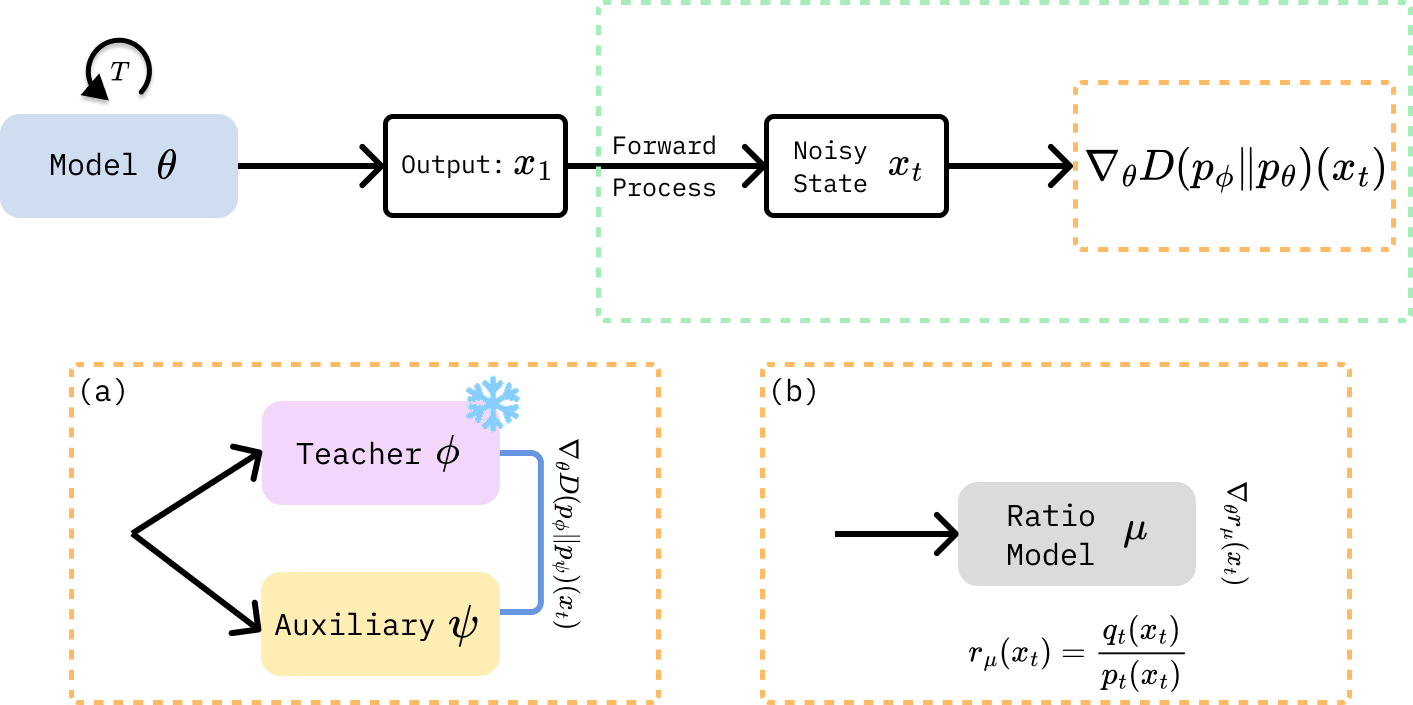
As shown in the above figure, the gradient of the divergence can be estimated in two ways: (a) the score-based approach (e.g., DMD) and (b) the discriminator-based approach (e.g., Diffusion GAN).

Diffusion Reinforcement Learning

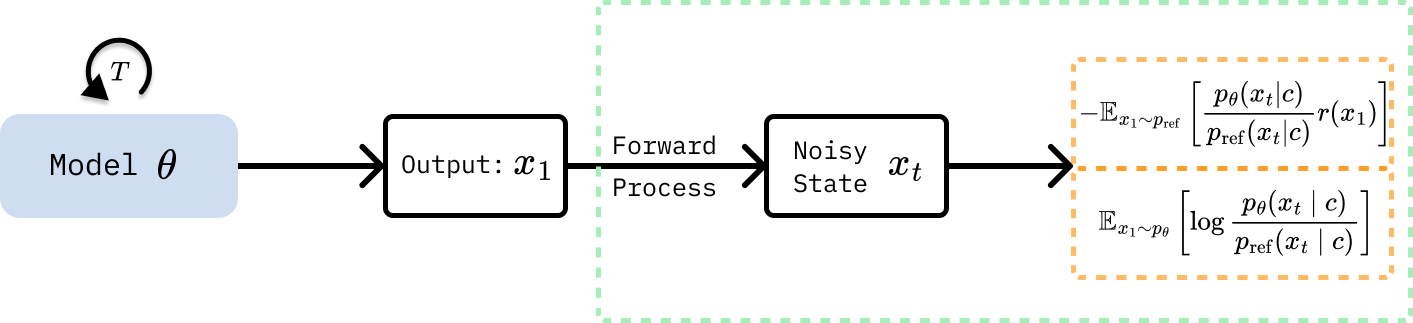
For diffusion RL fine-tuning, the target distribution is usually defined with a reference model and a reward model, which can be seen as a Boltzmann distribution $p_{\mathrm{target}}(x_1\mid c, c_\mathrm{ext}) \propto p_{\mathrm{ref}}(x_1\mid c) \exp(r(x_1))$, where $r(x_1)$ is the reward function defined by the reward model.

In this case, the objective can be written as:

$$ \begin{align*} \mathcal{L}(\theta) % &= \mathbb{E}_{x_0, c} \left[ D(p_\theta(x_1\mid c) \| p_{\mathrm{target}}(x_1\mid c)) \right] \\ &= \mathbb{E}_{x_0, c} \left[ D(p_{\mathrm{ref}}(x_1\mid c) \exp(r(x_1)) \| p_\theta(x_1\mid c)) \right] \end{align*} $$

Expanding using reverse KL divergence and splitting the log:

$$ \begin{align*} \mathbb{E}_{x_0, c} \left[ \mathbb{E}_{x_1 \sim p_\theta} \left[ \log \frac{p_\theta(x_1 \mid c)}{p_{\mathrm{ref}}(x_1 \mid c)} - r(x_1) \right] \right] \end{align*} $$

Splitting the expectation and rearranging terms, we have two terms: the reward term $\mathbb{E} _ {x_1 \sim p_\theta}[-r(x_1)]$ and the KL regularization term $\mathbb{E} _ {x_1 \sim p_\theta} \left[ \log \frac{p_\theta(x_1 \mid c)}{p_{\mathrm{ref}}(x_1 \mid c)} \right]$. With importance sampling and the REINFORCE log-derivative trick $\nabla_\theta \mathbb{E} _ {p_\theta}[f] = \mathbb{E} _ {p_\theta}[f \cdot \nabla_\theta \log p_\theta] $, we can rewrite the reward term as $\mathbb{E} _ {x_1 \sim p_{\mathrm{ref}}} \left[ - \frac{p_\theta(x_1 \mid c)}{p_{\mathrm{ref}}(x_1 \mid c)} r(x_1) \right]$.

As a result, the objective can be rewritten as a standard RL objective with KL regularization:

$$ \begin{align*} \boxed{\mathcal{L}(\theta) \propto -\mathbb{E}_{x_1 \sim p_{\mathrm{ref}}} \left[ \frac{p_\theta(x_1 \mid c)}{p_{\mathrm{ref}}(x_1 \mid c)} r(x_1) \right] + \mathbb{E}_{x_1 \sim p_\theta} \left[ \log \frac{p_\theta(x_1 \mid c)}{p_{\mathrm{ref}}(x_1 \mid c)} \right]} \end{align*} $$

For diffusion model, the density ratio $p_\theta / p_{\mathrm{ref}}$ can be estimated by the diffusion ELBO estimator, which is the same as the weighted denoising score matching (DSM) loss. To be specific, in the ELBO estimator, we calculate the density ratio at a randomly sampled time step $t$ as $r_t(x_t) = \frac{p_{\theta,t}(x_t|c)}{p_{\mathrm{ref},t}(x_t|c)}$, where $q_{\theta,t}$ is the generator marginal and $p_{\mathrm{ref},t}$ is the reference model marginal at time step $t$. The diffusion RL training can be summarized in the below figure.

Summary

In this blog, we show that diffusion distillation and diffusion RL fine-tuning are both instances of on-policy distillation, minimizing a divergence $D(p_{\mathrm{target}} | p_\theta)$, differing mainly in the choice of target distribution and the approach to estimate the divergence.

Acknowledgements

The author thanks Yuchen Zhu for his insightful discussion.