Bayesian Posterior Sampling (1) Introduction

The last post was written around one year ago, when I decided to switch my semester project topic from style transfer with normalizing flow to image restoration with diffusion models.

In my current engineering-oriented master’s thesis, I find myself longing for the elegance of the theory of diffusion models. As a solution, I have made the decision to dedicate my spare time to learning Bayesian sampling (sampling method for bayesian inference).

Hence I will write a series of posts to record this learning process and to improve my understanding of this topic by reorganizing my knowledge. In this post, I will start with some basics and a brief introduction to this topic.

Introduction

Bayesian Inference Problem & Challenging

Bayes Theorem
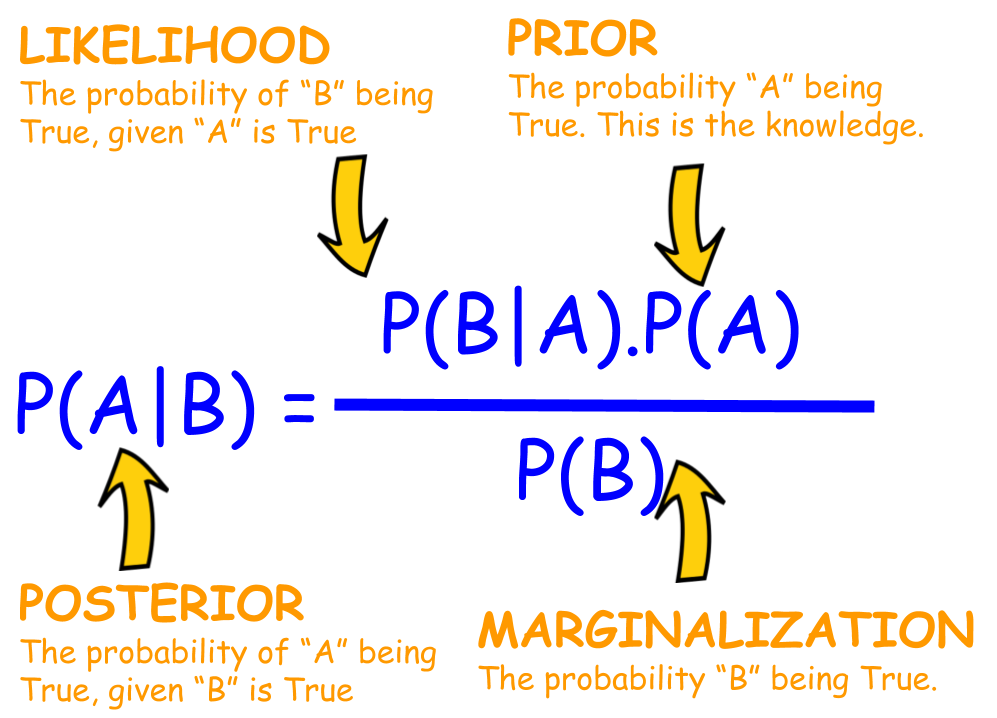
Figure 1: Visual Representation of Bayes' Theorem.

In the probabilistic approach to machine learning, all unknown quantities — be they predictions about the future, hidden states of a system, or parameters of a model — are treated as random variables, and endowed with probability distributions. The process of inference corresponds to computing the posterior distribution over these quantities, conditioning on whatever data is available.

—— Probabilistic Machine Learning: Advanced Topics by Kevin Patrick Murphy. MIT Press, 2023.

To be specific, we assume the dependence between unknown random latent variable $z$ and the available data $x$ is probabilistic and what we want to do is to estimate $z$ given $x$ with $p(z| x)$, which we call posterior. Most of the time we only have some prior knowledge about $z$ as $p(z)$ and the likelihood model $p(x|z)$, or equivalently the deep latent variable model $p_\theta(x, z)=p_\theta(z)p_\theta(x|z)$ through Bayesian Modeling, where $\theta$ can be estimated with maximizing likelihood (Maximizing the expected log-likelihood is equivalent to minimizing the Kullback-Leibler (KL) divergence between $p_{\mathrm{data}}(\mathbf{x})$ and $p_{\theta}(\mathbf{x})$):

$$ \begin{align} -\mathbb{E}_{\mathbf{x}\sim p_{\mathrm{data}}(\mathbf{x})}\left[\log p_\theta(\mathbf{x})\right] &= D_{K L}(p_{\mathrm{data}}(\mathbf{x})\lVert p_{\theta}(\mathbf{x}))\underbrace{-\mathbb{E}_{\mathbf{x}\sim p_{\mathrm{data}}(\mathbf{x})} \left[ \log p_{\mathrm{data}}(\mathbf{x})\right]}_{\text{constant}} \\ &\approx \prod_{n=1}^{N}\log p_\theta(x_{n}) = \prod_{n=1}^{N}\log [\int p_\theta(z_{n})p_\theta(x_{n}|z_{n})dz_{n}] \label{likelihood}\tag{1} \\ \end{align} $$

where the constant term is the entropy of the data distribution. While the entropy of the empirical data distribution goes to infinity, it is independent of $\theta$ and can be ignored in optimization.

We can compute the posterior $p_{\theta}(z| x)$ using Bayes’s rule (see Figure 1 for visual illustration):

$$ \begin{align} p_{\theta}(z|x)&=\frac{p_{\theta}(x|z)p_{\theta}(z)}{p_{\theta}(x)}\label{bayes}\tag{2} \\ \end{align} $$

where the evidence term (also called marginal likelihood) served as a normalization constant in the denominator can be formulated as:

$$ \begin{align} p_{\theta}(x)=\int p_{\theta}(x,z)dz=\int p_{\theta}(x|z)p_{\theta}(z)dz\label{evidence}\tag{3} \\ \end{align} $$

Beyond point estimation (MLE, MAP), we can use the posterior distribution to get posterior expectations of any function $f(z)$, such as mean and marginals. For instance, predicting new output in Bayesian linear regression where $w$ represents the coefficient that we aim to estimate its posterior distribution given the data: $y^\star =\int p(y^\star|x^\star, w)p(w | X,y)dw$.

However, this integral is usually analytically intractable¹ to calculate or evaluate, which leads to intractable posterior, and most Bayesian inference requires numerical approximation of such intractable integrals.

Two Approaches: Variational Inference & (MCMC) Sampling

In this post, I go through the two primary methodologies utilized to address the problem of Bayesian inference: Variational Inference (VI) and Markov Chain Monte Carlo (MCMC). I will strive to cover the most significant concepts associated with VI, and also provide a brief introduction to MCMC.

Variational Inference

Variational inference (VI) is a method in machine learning that approximates complex probability distributions by finding the most similar, simpler and hence tractable distribution $q(z)$ from a specified family $\mathcal{Q}$, thereby enabling efficient computation and handling of uncertainty.

Most of the time when referring to Variational Inference (VI), we are discussing parametric VI. In parametric VI, we use a parameter $\phi$ to represent the variational distribution $q_\phi(z|{x})$. There is another type of VI called particle-based VI, which utilizes a set of particles $\{z^{(i)}\}_{i=1}^{N}$ to represent the variational distribution $q(z|{x})$.

variational_inference
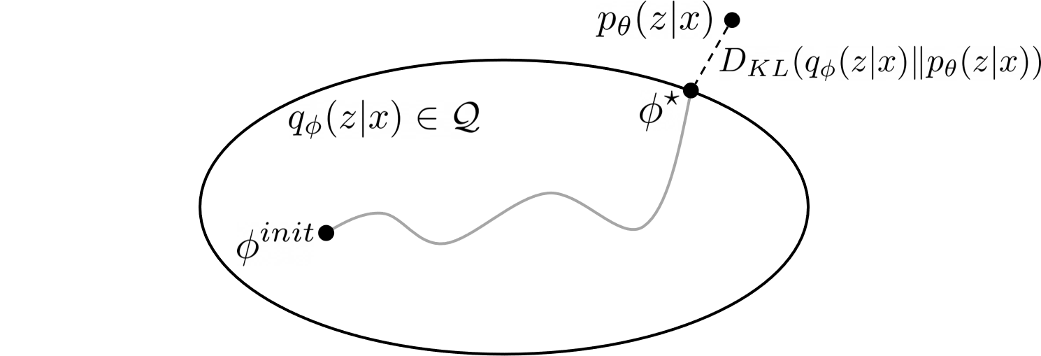
Figure 2: Illustration of Variational Inference.

The main idea of variational methods is to cast inference as an optimization problem. The goal of VI is to approximate an intractable probability distribution, so as to find $q_{\phi} \in \mathcal{Q}$ that minimize some discrepancy $D$ (here we use the KL divergence) between $q_{\phi}({z}|{x})$ and $p_{\theta}({z}|{x})$:

$$ \begin{align} q^{\star}_{\phi} = \underset{q_{\phi}\in \mathcal{Q}}{\operatorname{\arg\min }} D_{K L}(q_{\phi}({z}|{x})\lVert p_{\theta}({z}|{x}))\label{KL}\tag{4} \\ \end{align} $$

The challenge here is that we still don’t know the true posterior $p_{\theta}({z}|{x})$, and the KL divergence is intractable to compute. Luckily, we can rewrite the KL divergence in a way that makes it easier to optimize:²:

$$ \begin{align*} D_{K L}(q_{\phi}({z}|{x})\lVert p_{\theta}({z}|{x}))&=\mathbb{E}_{q_{\phi}({z}|{x})}\left[\log\left[\frac{q_{\phi}({z}|{x})}{p_{\theta}({z}|{x})}\right]\right] \\ &=\mathbb{E}_{q_{\phi}({z}|{x})}\left[\log\left[\frac{q_{\phi}({z}|{x})p_{\theta}({x})}{p_{\theta}({x},{z})}\right]\right] \\ &=\mathbb{E}_{q_{\phi}({z}|{x})}\left[\log\left[\frac{q_{\phi}({z}|{x})}{p_{\theta}({x},{z})}\right]\right] + \mathbb{E}_{q_{\phi}({z}|{x})}\left[\log p_{\theta}({x})\right]\\ &=\mathbb{E}_{q_{\phi}({z}|{x})}\left[\log\left[\frac{q_{\phi}({z}|{x})}{p_{\theta}({x},{z})}\right]\right] + \log p_{\theta}({x})\label{KL_derivation}\tag{5}\\ \end{align*} $$

where the log evidence $\log p_\theta({x})$ does not change with the choice of $\phi$ during variational inference.

For convention, we can rewrite this as:

$$ \begin{align*} \log p_\theta({x})=\mathbb{E}_{q_{\phi}({z}|{x})}\left[\log\left[\frac{p_{\theta}({x},{z})}{q_{\phi}({z}|{x})}\right]\right]+\underbrace{D_{K L}(q_{\phi}({z}|{x})\lVert p_{\theta}({z}|{x}))}_{\geq 0} \label{evidence2}\tag{6} \end{align*} $$

Since the KL divergence between $q_{\phi}({z}|{x})$ and $p_{\theta}({z}|{x})$ is non-negative, the first term in the RHS of eq(\ref{evidence2}) is a lower bound of the log evidence term $\log p_\theta({x})$, which is named variational lower bound, also called the Evidence Lower BOund (ELBO):

$$ \begin{align*} \mathcal{L}_{\theta,\phi}({x})=\mathbb{E}_{q_{\phi}({z}|{x})}\left[\log p_{\theta}({x},{z})-\log q_{\phi}({z}|{x})\right]\label{ELBO}\tag{7} \end{align*} $$

Therefore, the common mission to find the optimal $q_{\phi}({z}|{x})$ that minimizes the KL divergence (approximates $p_{\theta}({z}|{x})$) is equivalent to maximize the ELBO (without worrying about the evidence term in $p_{\theta}({z}|{x})$), and we can optimize it w.r.t. both ${\phi}$ and ${\theta}$ (when $\theta$ is unknown) in algorithms such as variational EM.

As $\theta$ is the model parameters, optimizing $\theta$ is essential for learning the underlying model that generates the data. When $\theta$ is tunable, we can jointly optimize $\phi$ and $\theta$ to maximize the ELBO. This joint optimization can help in finding a more accurate posterior approximation ($\phi$) and model parameters that better explain the data ($\theta$ that gives tighter ELBO of likelihood).

²We can also get the same ELMO starting from the KL divergence between joint distributions $D_{KL}(q_{\phi}({x},{z})\lVert p_{\theta}({x},{z}))$, see this blog by Jianlin Su and this blog by Alex Alemi.

³It's recommended to read this blog by Casey Chu and this famous paper ELBO surgery by Matthew D. Hoffman and Matthew J. Johnson for more perspectives on the ELBO.

⁴For VAE, there is a great introduction by D.P. Kingma and Max Welling.

⁵For a comprehensive understanding of advanced concepts in VAE such as the $\beta$-VAE, I highly recommend reading Lilian Weng's blog.

⁶This great blog by Alex Alemi also derives the diffusion loss through variational perspective for those who are interested in diffusion models.

We can rewrite the ELBO as follows³:

$$ \begin{align*} \mathcal{L}_{\theta,\phi}({x}) &= \underbrace{\mathbb{E}_{q_{\phi}({z}|{x})}[\log p_{\theta}({x},{z})]}_{\text{expected log joint}}+\underbrace{\mathbb{H}(q_{\phi}({z}|{x}))}_{\text{entropy}}\label{ELBO2}\tag{8} \end{align*} $$

Additionally, the ELBO can be reorganized and interpreted as the following in Variational AutoEncoder (VAE)⁴^,⁵, where $\phi$ and $\theta$ represent the encoder and decoder, respectively:

$$ \begin{align*} \mathcal{L}_{\theta,\phi}({x}) &= -[\underbrace{\mathbb{E}_{q_{\phi}({z}|{x})}[-\log p_{\theta}({x}|{z})]}_{\text{expected negative log likelihood}}+\underbrace{D_{K L}(q_{\phi}({z}|{x})\lVert p_{\theta}({z}))}_{\text{KL from posterior to prior}}] \\ &=-\mathbb{E}_{q_{\phi}({z}|{x})}[\underbrace{-\log p_{\theta}({x}|{z})}_{\text{reconstruction error}}+\underbrace{\log q_{\phi}({z}|{x})-\log p_{\theta}({z})}_{\text{regularization (align) terms}}] \label{ELBO3}\tag{9}\\ \end{align*} $$

Suppose $p_{\theta}({x}|{z})=\mathcal{N}(\mu_\theta(z),\sigma^2)$, and $q_{\phi}({z}|{x})$ is a deterministic mapping $\psi_{\phi}(x)$. The first term is a reconstruction error, proportional to $|| x−\mu_\theta(\psi_{\phi}(x))||^2$. And the training objective on given dataset is hence⁶:

$$ \begin{align*} \mathbb{E}_{\mathbf{x}\sim p_{\mathrm{data}}(\mathbf{x})}[\mathcal{L}_{\theta,\phi}({x})] = -\mathbb{E}_{\mathbf{x}\sim p_{\mathrm{data}}(\mathbf{x})}\mathbb{E}_{\mathbf{z}\sim q_{\phi}({z}|{x})}[-\log p_{\theta}({x}|{z})+\log q_{\phi}({z}|{x})-\log p_{\theta}({z})] \label{objective}\tag{10} \end{align*} $$

The optimization of the above equation (\ref{objective}) usually involve taking gradient w.r.t. $\phi$, which is more difficult as we cannot swap the gradient and the expectation like when taking gradient w.r.t. $\theta$. To resolve this issue, we can use methods like score function estimator and the reparametrization trick.

Markov Chain Monte Carlo

Unlike VI which solves inference with optimization, MCMC tackles it via sampling techniques. More specifically, MCMC applies Monte Carlo methods to generate a sufficient number of samples for an accurate estimation of the posterior distribution. However, it is almost always impossible to directly do so. As a solution, we can use MCMC, which is aimed at simulating a Markov chain whose stationary distribution is $p_{\theta}({z}|{x})$ and hope a fast convergence. And guess what, we only need unnormalized probability density (e.g. $p(x,z)$) to simulate the chain!

Optimization: find the minimum $min_{x\in \mathbb{R}^d} U(x)$

Sampling: draw samples from the density $\pi(x)\propto e^{-U(x)}$

A more general problem setting is: sampling (=generating new examples) from a target distribution $\pi$ over $\mathbb{R}^d$ whose density is known up to an intractable normalization constant $Z$⁷:

$$ \begin{align*} \pi(x) &= \frac{1}{Z}\tilde{\pi}= \frac{\exp(-\beta U(x))}{Z} \label{target_dist}\tag{11}\\ \end{align*} $$

where $\tilde{\pi}$ is the known unnormalized distribution, $\beta$ is an arbitrary positive constant akin to an inverse temperature, and $U(\cdot)$ can be treated as energy function. To make the notation consistent, now we rewrite the problem (\ref{KL}) as:

$$ \begin{align*} \pi^\star = \underset{\mu\in \mathcal{P}_2(\mathbb{R}^d)}{\operatorname{\arg\min }} D(\mu \lVert \pi) := \mathcal{F}_\pi(\mu)\label{KL_MCMC}\tag{12} \\ \end{align*} $$

where $D$ is a dissimilarity functional such as KL divergence, and $\mathcal{F}_{\pi}(\mu)$ is a shorthand of $D(\mu \lVert \pi)$. We can approximate integrals $\int f(\cdot) d\pi$ of any function $f(\cdot)$ with samples from the Markov chain as $\frac{1}{n}\Sigma_{i=b}^{b+n-1}f(x_i)$, where $b,n$ are sufficiently large integers, and $b$ is called the mixing time or burn-in time. Note that the initial samples from the chain should be discarded because they do not come from the stationary distribution; reducing this is one of the most important factors in securing a fast convergence.

The ultimate goal of this series of posts is exactly to learn various MCMC techniques to sample from $\pi^\star$!
It’s also highly recommended to try out this great website for fantastic MCMC animations first.

The future topics should include: