Prerequisite: Normalizing Flow

Overview

Normalizing Flow (NF) is a kind of generative model just like GANs and VAEs but provides injective mapping between data $X$ and latent variable $Z$ (from a simple distribution) with exact likelihood calculations. Among all the NFs, real NVP is one of the most important, which stands for real-valued non-volume preserving (real NVP) transformation, a set of powerful invertible and learnable transformations.

Target: The goal here is to build a learnable, reversible transformation between a source domain (distribution) and a latent (simple distribution) domain $Z$ or another target domain. Just like most of the other NFs, we can train the real NVP by doing maximum likelihood estimation (MLE).

From now on we just consider the following situation: source domain is images of a style and target domain is Gaussian distribution.

We need to first write the likelihood of source images $p_X(X)$ in a form that is easy to compute. Given an image $x \in X$, a simple prior probability distribution $p_Z$ on a latent variable $z \in Z$, and a bijection $f : X \rightarrow Z$ (with $g = f^{−1}$ ), the change of variable formula defines a model distribution on $X$ by (as we assume $p_Z$ is Gaussian):

where $p_Z(f(x))$ is easy to get given $z=f(x)$, $\mid \text{det}(\frac{\partial f(x)}{\partial x^T})\mid$ is the determinant of Jacobian, which can be construct to be computational efficient, too.

$f$ can be decomposed to many invertible component: $f = f_1 \circ f_2 \circ … \circ f_n$ just like deep neural network.

We describe here a batch of images as tensor of size $\text{batch}.\text{size}() = (B,C,H,W)$.

For simplicity, we set batch_size $B=1$. For any input image, we expect to get a latent variable $z\sim N(0,1)$. In order to calculate $\text{log} p_X(x)$, the model is also required to keep track the sum of log determinant of Jacobian (sldj) $J = \log \det \frac{\partial f(x)}{\partial x^T}$.

Pre-process

We further assume the value of each element in this tensor $\in [0,1]$.

The next step is to de-quantize these images, to make the values a continues distribution. (Since the discrete data distribution has differential entropy of negative infinity, this can lead to arbitrary high likelihoods even on test data. To avoid this case, it is becoming best practice to add real-valued noise to the integer pixel values to de-quantize the data):

x = (x * 255. + torch.rand_like(x)) / 256.      # [0,1] with noise

Notice: now for the same input images, the model will give each time slightly different $z\in Z$.

According to https://arxiv.org/abs/1605.08803, Section 4.1, we will model logits $y = \log(x) - \log(1 - x)$:

y = x.log() - (1. - x).log()            

Since $x\in [0,1]$, it’s dangerous to apply directly log to them, so we apply a data_constraint $\beta=0.9$ to $x$:

# Convert to logits
y = (2 * x - 1) * self.data_constraint  # [-0.9, 0.9]
y = (y + 1) / 2                         # [0.05, 0.95]
y = y.log() - (1. - y).log()            # logit: y=log((((2x-1)beta+1)/2)/(1-((2x-1)beta+1)/2))          

Now let compute the sldj of pre-process step.

# Save log-determinant of Jacobian of initial transform
# Softplus(x) = 1/beta*log(1+exp(beta*x)) (default beta=1) element-wise: activation function
ldj = F.softplus(y) + F.softplus(-y) \
    - F.softplus((1. - self.data_constraint).log() - self.data_constraint.log())
# sum up pixels and channels of every in each batch
ldj = ldj.view(ldj.size(0), -1).sum(-1)

As commented above, $\text{F.softplus}(x) = \text{log}(1+e^{x})$, and it’s obvious that $\text{F.softplus}(\text{log}(1-\beta)-\text{log}(\beta)) = \text{log}(1/\beta)$.

For $\text{F.softplus}(y) + \text{F.softplus}(-y)$, the reader can verify it is correct themselves or go through the next few lines.

Real NVP model

Coupling Layer

The very key component of Real NVP is the coupling layer, which is used to passing information while keep the sldj easy to compute. The original figure of coupling from the paper illustrates the forward and inverse operation of this coupling layer. In this coupling layer, the input $x$ is split into two $x_1$ and $x_2$ by channel, and then propagates according to this figure.

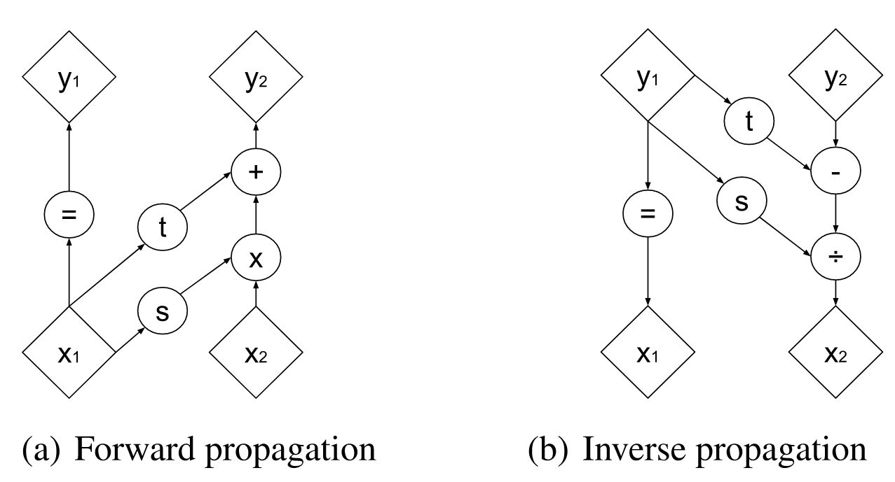
Indeed, this figure is about the so called affine coupling layer (with scale and bias terms), where the functions $s$ and $t$ can be arbitrary complex neural networks (even attention module or with additional/conditional information injected).

# split x
x_change, x_id = x.chunk(2, dim=1)
st = self.nn(x_id)
# apply the nn in a checkerboard manner
s, t = st[:, 0::2, ...], st[:, 1::2, ...]
s = self.scale * torch.tanh(s)
# Scale and translate
if reverse:
    x_change = x_change * s.mul(-1).exp() - t
    # track ldj
    ldj = ldj - s.flatten(1).sum(-1)
else:
    x_change = (x_change + t) * s.exp()
    # track ldj
    ldj = ldj + s.flatten(1).sum(-1)
# concatenate recover x
x = torch.cat((x_change, x_id), dim=1)

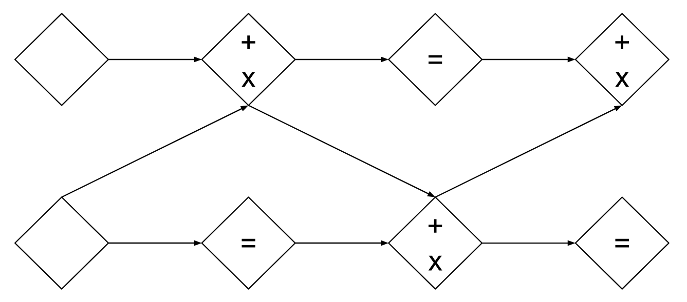
This structure is invertible because $y_1=x_1$ is guaranteed for both forward and inverse propagation. On the other hand, this also means that the we can’t keep those channels unchanged all the time. One way to do so is to swap the position of $x_1$ and $x_2$ recursively like in the figure below. (in Glow model, the $1\times 1$ invertible convolution is introduced to better mitigate this issue.)

Squeezing and Masking

Before the coupling layer, the checkerboard masking and squeezing is introduced, as shown in the following figure:

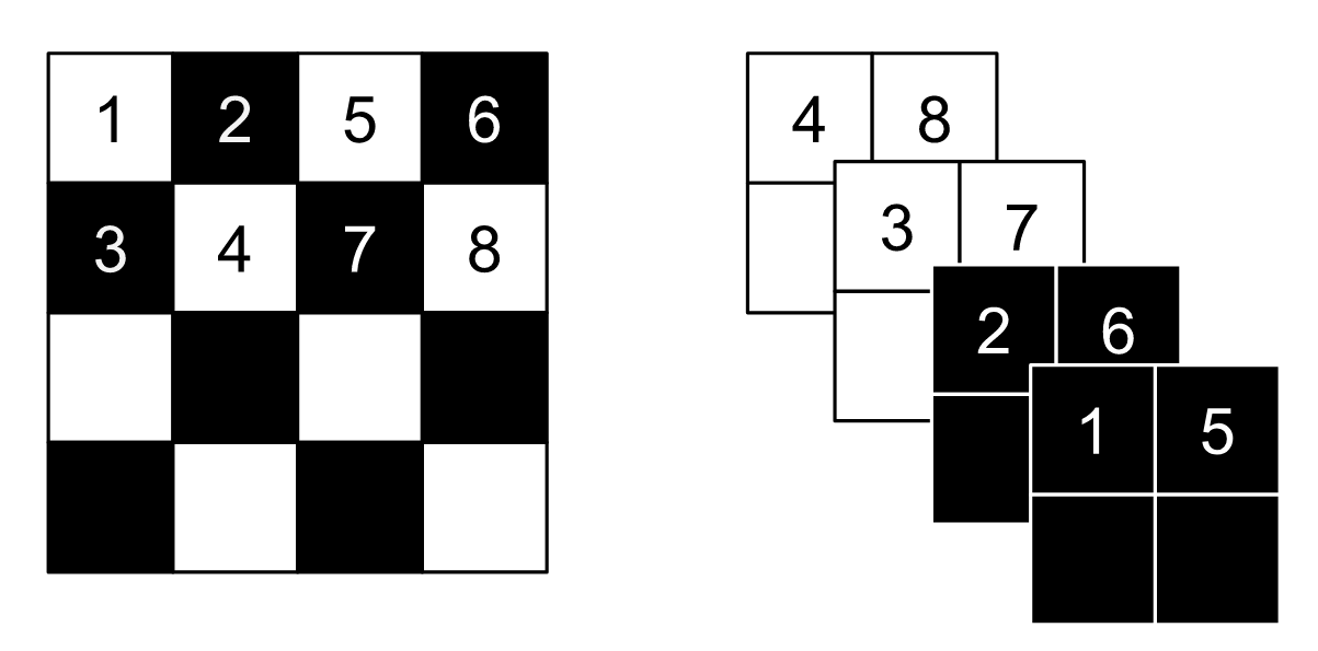
As you may get from this figure, each sub-channel after squeezing is just a scaled smaller image. This makes suer that $x_1$ and $x_2$ contain the information from the original image evenly.

According to the original paper: The squeezing operation reduces the $4 × 4 × 1$ tensor (on the left) into a $2 × 2 × 4$ tensor (on the right). Before the squeezing operation, a checkerboard pattern is used for coupling layers while a channel-wise masking pattern is used afterward.

These operations are both invertible because they are both linear operations.

Multi-scale Architecture

The squeeze operation mentioned above enable a multi-scale architecture used in the Real NVP, as shown in this picture. The main purpose of this architecture is to save computational resources (GPU memory etc.). When initializing the model, each scale is initialized recursively.

# recursively build real NVP scales 
if num_scales > 1:
    self.next = _RealNVP(*args,num_scales=num_scales - 1)

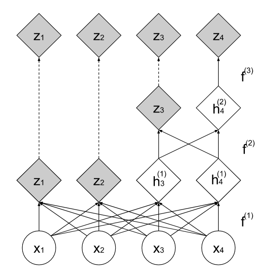
As you can see in the figure, in each scale the size of the image is halved but with full connection to the next scale(information passing).

x = squeeze(x)
# split
x, x_split = x.chunk(2, dim=1)
x, sldj = self.scale(x, sldj, reverse)
# cat
x = torch.cat((x, x_split), dim=1)
x = squeeze(x, reverse=True)

Every time after the squeeze, $x$ is split into $x$ and $x_{split}$, where $x$ will be processed in the following scale blocks and $x_{split}$ will remain unchanged. After $x$ is processed, it’s concatenated with $x_{split}$ to form the output with same size.

References

https://uvadlc-notebooks.readthedocs.io/en/latest/tutorial_notebooks/tutorial11/NF_image_modeling.html